Chapter 10 Poisson processes
The Poisson process is a model for counting the number of events that have occurred up to time \(t\). It is a continuous-time stochastic process \[ X=(X_t)_{t\in[0,\infty)} \] where \(X_t\) is the number of events that have occurred in the time interval \([0,t]\). We assume \(X_0=0\), so the counter starts at zero.
There is a single parameter \(\lambda>0\), called the rate parameter, intensity, or arrival rate. It represents the average number of events per unit time. If events arrive at rate \(\lambda\), then the number of events in a time interval of length \(t\) is Poisson distributed with mean \(\lambda t\): \[ X_t\sim\mathsf{Pois}(\lambda t). \]
Before defining the Poisson process carefully, we review the exponential, gamma, and Poisson distributions.
10.1 Exponential distribution
Let \(X\sim\mathsf{Exp}(\lambda)\), where \(\lambda>0\) is the rate parameter. The probability density function is \[ f_X(t)=\lambda e^{-\lambda t},\quad t>0, \] and the cumulative distribution function is \[ F_X(t)=1-e^{-\lambda t},\quad t>0. \] The mean and variance are \[ \mathbb E(X)=\frac1\lambda,\qquad \mathsf{Var}(X)=\frac1{\lambda^2}. \]
Sometimes the exponential distribution is parametrized by its mean \(\alpha=1/\lambda\) instead of its rate. In that convention, \[ f_X(t)=\frac1\alpha e^{-t/\alpha},\quad t>0. \]
The exponential distribution is often used to model waiting times. For example, it can model the time between insurance claims, the time between arrivals in a customer service queue, the lifetime of a radioactive particle, or the time between births or deaths in a population.
10.2 Memorylessness
The exponential distribution has the memoryless property: \[ \mathbb P(X>t+s\mid X>s)=\mathbb P(X>t), \] for \(s,t\geq0\). In words, if we have already waited \(s\) units of time, then the additional waiting time is still exponentially distributed with the same rate.
To verify this, calculate \[ \begin{aligned} \mathbb P(X>t+s\mid X>s) &=\frac{\mathbb P(X>t+s, X>s)}{\mathbb P(X>s)}\\ &=\frac{\mathbb P(X>t+s)}{\mathbb P(X>s)}\\ &=\frac{e^{-\lambda(t+s)}}{e^{-\lambda s}}\\ &=e^{-\lambda t}\\ &=\mathbb P(X>t). \end{aligned} \]
Memoryless property. If \(X\sim\mathsf{Exp}(\lambda)\), then \[ \mathbb P(X>t+s\mid X>s)=\mathbb P(X>t). \] This is one reason the exponential distribution is the natural continuous-time analogue of the geometric distribution.
10.3 Conditional expectation for exponential waiting times
The memoryless property also implies that \[ \mathbb E(X\mid X>s)=s+\frac1\lambda. \] This says that if we know the event has not occurred by time \(s\), then our expected total waiting time is the time already waited plus one fresh exponential mean.
We can derive this directly. For \(t\geq s\), \[ \begin{aligned} F_{X\mid X>s}(t) &=\mathbb P(X\leq t\mid X>s)\\ &=\frac{\mathbb P(s<X\leq t)}{\mathbb P(X>s)}\\ &=\frac{e^{-\lambda s}-e^{-\lambda t}}{e^{-\lambda s}}\\ &=1-e^{-\lambda(t-s)}. \end{aligned} \] Thus the conditional density is \[ f_{X\mid X>s}(t)=\lambda e^{-\lambda(t-s)},\quad t>s. \] So \(X\mid X>s\) has the same distribution as \(s+Z\) where \(Z\sim\mathsf{Exp}(\lambda)\). Therefore, \[ \mathbb E(X\mid X>s)=s+\mathbb E(Z)=s+\frac1\lambda. \]
10.4 Gamma distribution
Let \(X\sim\Gamma(n,\lambda)\) with shape parameter \(n\) and rate parameter \(\lambda\). For \(n=1,2,3,\ldots\), the density is \[ f_X(t)=\frac1{\Gamma(n)}(\lambda t)^{n-1}\lambda e^{-\lambda t},\quad t>0. \] When \(n\) is a positive integer, \[ \Gamma(n)=(n-1)!. \]
If \(X_1,X_2,\ldots,X_n\) are independent exponential random variables with rate \(\lambda\), then \[ \sum_{j=1}^n X_j\sim\Gamma(n,\lambda). \] For a Poisson process, this will represent the waiting time until the \(n^{th}\) event.
Gamma waiting time interpretation. If events arrive one at a time and the waiting times between events are i.i.d. \(\mathsf{Exp}(\lambda)\), then the waiting time for the \(n^{th}\) event has distribution \(\Gamma(n,\lambda)\).
10.5 Poisson distribution
Let \(N\sim\mathsf{Pois}(\lambda)\). Then \[ \mathbb P(N=k)=e^{-\lambda}\frac{\lambda^k}{k!},\quad k=0,1,2,\ldots. \] The mean and variance are both equal to \(\lambda\): \[ \mathbb E(N)=\mathsf{Var}(N)=\lambda. \]
The Poisson distribution models the number of events occurring in a unit of time or space. If events occur at rate \(\lambda\) per unit time, then the number of events in \(t\) units of time is \[ \mathsf{Pois}(\lambda t). \]
A useful way to compare the binomial and Poisson distributions is this: the binomial counts successes over a discrete set of trials, while the Poisson counts events over a continuous interval of time or space.
10.6 Definition of the Poisson process
A stochastic counting process \((X_t)_{t\geq0}\) is a Poisson process with rate \(\lambda\) if:
- \(X_0=0\),
- \(X_t\) has independent increments over non-overlapping time intervals,
- the number of arrivals in an interval of length \(t\) has distribution \(\mathsf{Pois}(\lambda t)\).
Thus, for \(0\leq s<t\), \[ X_t-X_s\sim\mathsf{Pois}(\lambda(t-s)). \] The independent increments assumption says that counts on disjoint intervals are independent.
We can also describe the process dynamically by saying \[ X_t\to X_t+1\quad\text{at rate }\lambda. \] That means that the process sits at its current value and waits an exponential amount of time with rate \(\lambda\), then jumps up by one.
10.7 Waiting time construction
Let \[ \tau_1,\tau_2,\tau_3,\ldots \] be i.i.d. exponential random variables with rate \(\lambda\). These are the additional waiting times between events. Define the arrival times \[ S_n=\tau_1+\tau_2+\cdots+\tau_n. \] Then \(S_n\sim\Gamma(n,\lambda)\). The Poisson process can be constructed by setting \[ X_t=n\quad\text{if}\quad S_n\leq t<S_{n+1}. \] Equivalently, \[ X_t=\max\{n:S_n\leq t\}. \]
Poisson process from exponential waiting times. If the interarrival times \(\tau_1,\tau_2,\ldots\) are i.i.d. \(\mathsf{Exp}(\lambda)\), then the process that counts how many arrivals have occurred by time \(t\) is a Poisson process with rate \(\lambda\).
The probability of no events in the next \(t\) units of time is \[ \mathbb P(X_{s+t}=X_s\mid X_s=k)=e^{-\lambda t}. \] More generally, \[ \mathbb P(X_{s+t}-X_s=m)=e^{-\lambda t}\frac{(\lambda t)^m}{m!}. \]
10.8 Examples
Example. Suppose insurance claims arrive at rate one every two hours. Then \(\lambda=1/2\) claims per hour.
The probability of no claims in the next five hours is \[ \mathbb P(\tau_1>5)=e^{-(1/2)5}=e^{-2.5}\approx0.0821. \]
The waiting time for the next five claims has distribution \[ \Gamma(5,1/2). \] Thus the probability that it takes less than seven hours for the next five claims to arrive is \[ \mathbb P(S_5<7)=\int_0^7 \frac1{4!}\left(\frac12 t\right)^4\frac12 e^{-t/2}\,dt. \] In R:
## [1] 0.274555- The number of claims in an eight-hour day is \[ X_8\sim\mathsf{Pois}\left(\frac12\cdot 8\right)=\mathsf{Pois}(4). \] So the probability of exactly five claims is \[ \mathbb P(X_8=5)=e^{-4}\frac{4^5}{5!}\approx0.1563. \] In R:
## [1] 0.156293510.9 Simulating a Poisson process in R
There are two convenient simulation methods.
10.9.1 Method 1: simulate exponential waiting times
We simulate exponential waiting times until the total time has exceeded a fixed horizon \(T\).
lambda <- 2
Tmax <- 5

waits <- rexp(1000, rate=lambda)
arrivals <- cumsum(waits)
arrivals <- arrivals[arrivals <= Tmax]

jump_times <- c(0, arrivals, Tmax)
counts <- c(0, seq_along(arrivals), length(arrivals))

plot(jump_times, counts, type="s", xlab="time", ylab="number of events")
points(arrivals, seq_along(arrivals), pch=20)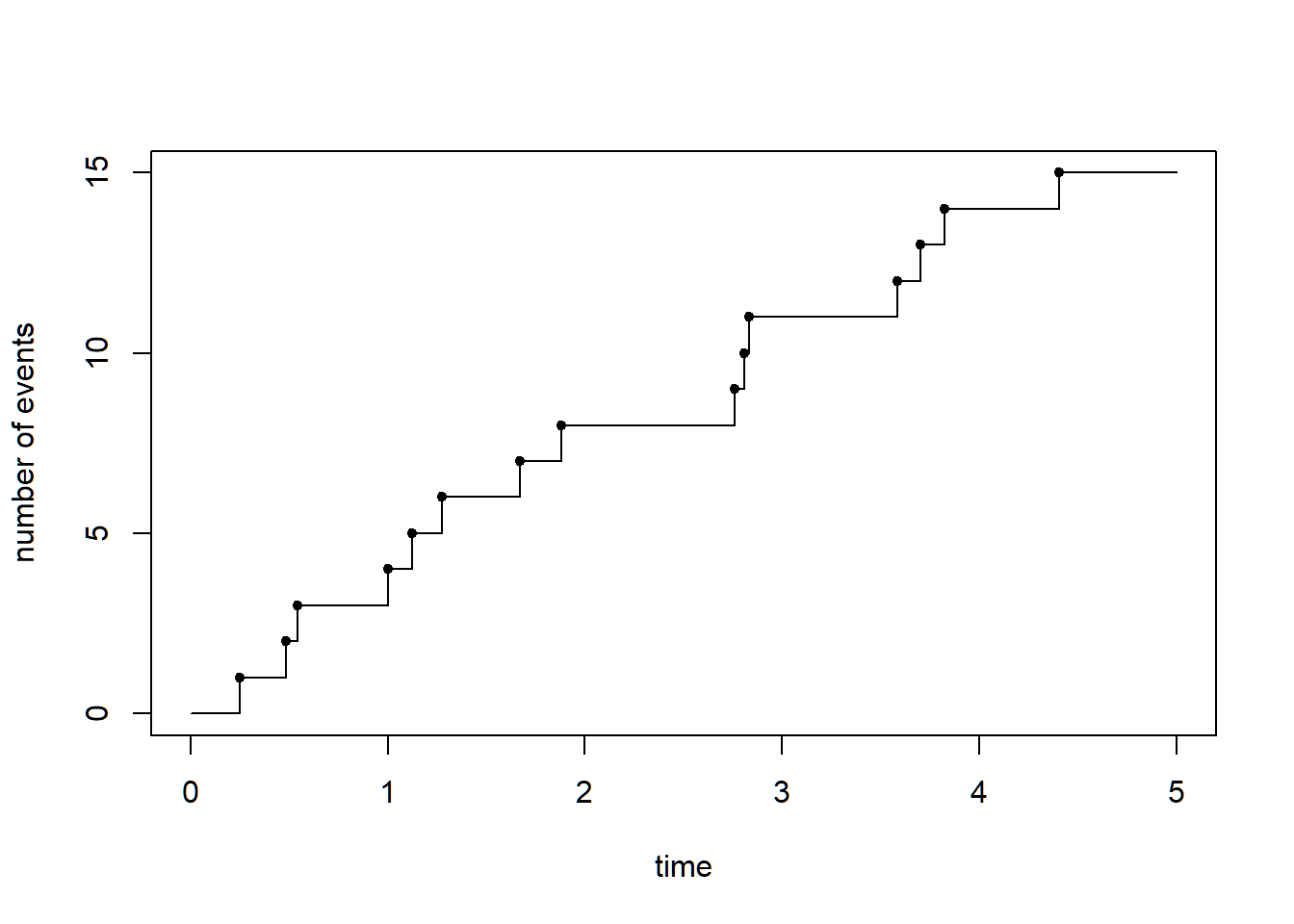
This produces a step function. The process stays constant between arrivals and jumps up by one at each arrival time.
10.9.2 Method 2: sample the number of points and place them uniformly
For a Poisson process on \([0,T]\), the total number of points is \[ N\sim\mathsf{Pois}(\lambda T). \] Conditional on \(N\), the \(N\) arrival times are distributed like independent uniform random variables on \([0,T]\), sorted into increasing order.
lambda <- 2
Tmax <- 5

N <- rpois(1, lambda*Tmax)
arrivals <- sort(runif(N, 0, Tmax))

jump_times <- c(0, arrivals, Tmax)
counts <- c(0, seq_along(arrivals), N)

plot(jump_times, counts, type="s", xlab="time", ylab="number of events")
points(arrivals, seq_along(arrivals), pch=20)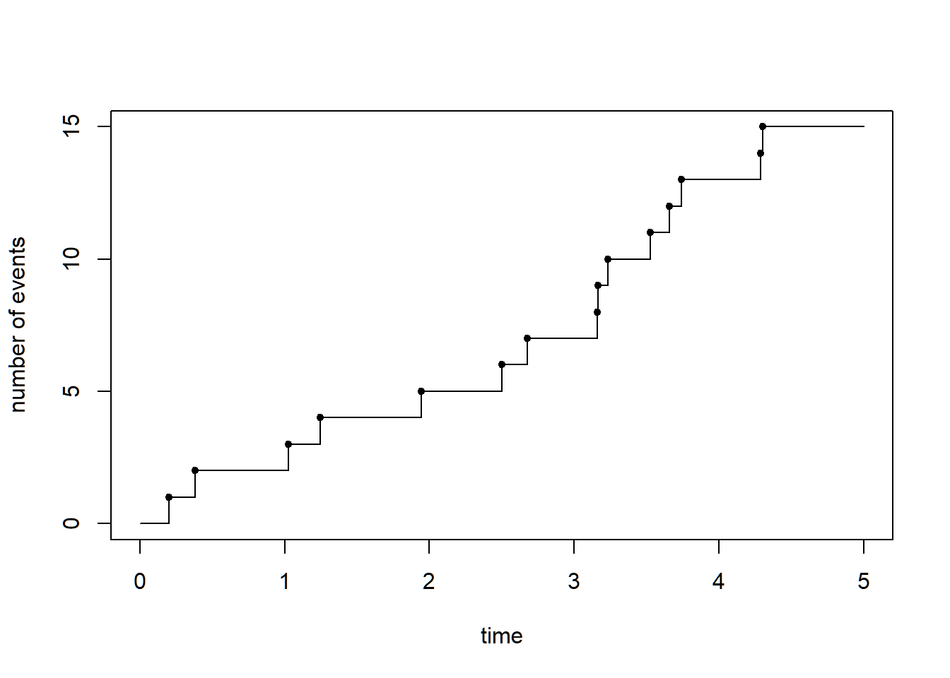
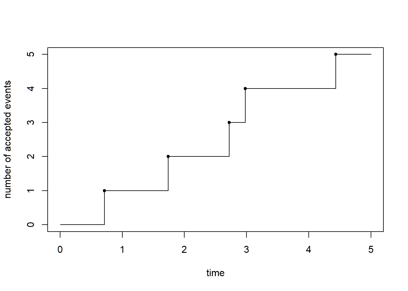
This method is especially useful for coupling Poisson processes with different rates. First simulate candidate points from a larger rate \(\lambda_{\max}\), then keep a candidate point for a smaller rate \(\lambda\leq\lambda_{\max}\) with probability \(\lambda/\lambda_{\max}\). This is called thinning.
lambda_max <- 4
lambda <- 1.5
Tmax <- 5

Nmax <- rpois(1, lambda_max*Tmax)
times <- runif(Nmax, 0, Tmax)
marks <- runif(Nmax, 0, lambda_max)
arrivals <- sort(times[marks <= lambda])

jump_times <- c(0, arrivals, Tmax)
counts <- c(0, seq_along(arrivals), length(arrivals))

plot(jump_times, counts, type="s", xlab="time", ylab="number of accepted events")
points(arrivals, seq_along(arrivals), pch=20)