Chapter 1 Introduction to R and RStudio

R is a statistical software package and a computer programming language. It is widely used in both industry (e.g. by data scientists) and academic research. RStudio is a graphical interface for R. Here I will give a brief introduction to R and RStudio.

1.1 Getting access to R and RStudio

There are two main ways to use R:

1. install R and RStudio locally on your computer, or

2. use Posit cloud. (Posit is the company that makes RStudio)

Posit Cloud:

I strongly suggest getting an account on Posit Cloud (this is the company that makes RStudio). Then you have access to a fully-capable and up-to-date version of R and RStudio form any web browser on any device. Go to: https://posit.cloud/, and sign up. Their free account simply has computation time limitations which should be no problem for most casual users.

Alternatively, you can download and install R and RStudio Desktop locally on your computer. I recommend doing this, especially if you are more serious about learning R or running programs that require more computation time.

Downloading and installing R statistical software:

I recommend two things:

1. Install R. This is the actual statistical software.

2. Install RStudio Desktop. This is a nice user interface for R.

*Note that the actual software version numbers change frequently, and they are, as of writing, R 4.2.2 and RStudio Desktop 2022.12.0+353.

Getting R:

First, download the appropriate version (Windows, Mac, etc.) of R from here: https://cloud.r-project.org/

For Windows:

• Click on “Download R for Windows”,

• then click on “install R for the first time”,

• then click on “Download R-4.2.2 for Windows”.

• Then install the software.

For Mac OS:

• Click on “Download R for macOS”,

• then click on either “R-4.2.2-arm64.pkg” or “R-4.2.2.pkg” (depending on macOS version and processor type).

• Then install the software.

I am more proficient at Windows than Mac, but if you have trouble installing it, come see me and I should be able to help you get it figured out. There are also Linux/Unix options—I am familiar with Ubuntu and so should be able to help on those platforms as well.

Getting RStudio Desktop:

After you have R installed, I recommend installing RStudio Desktop in order to have access to a more friendly user interface. I will always be using RStudio when I show demonstrations in class. Simply go here: https://posit.co/download/rstudio-desktop/#download and choose your desired version. The webpage should automatically detect your operating system and provide you with a link to the correct version of RStudio. You can scroll down the page and see links to various versions though. For Windows, the first link should work: “Windows 10/11 RSTUDIO-2022.12.0-353.EXE”. For MacOS the second link should work: “macOS 11+ RSTUDIO-2022.12.0-353.DMG”. Install the software. Done! There is also a link for older versions of RStudio in case you have an older version of Windows, MacOS, or Linux, etc.

Brief test of R & RStudio:

Launch RStudio Desktop or open a Posit Cloud Workspace/Project. Locate the “Console” subwindow. This is where we will type our commands. Type x <- 3 in the console next to the “>” (which is a command prompt that you will always type command next to). Then press the enter or return key on your keyboard. This saves the value of 3 for the variable x. Then type x+5 and hit enter. You should see the output [1] 8. This indicates the result of the computation. The “[1]” indicates that the output is a single number. Later on we will learn many interesting commands that are useful. Now you know how to open RStudio and use it as a calculator!

The RStudio user interface is shown below. The most important parts are highlighted and labeled wtih brief descriptions.

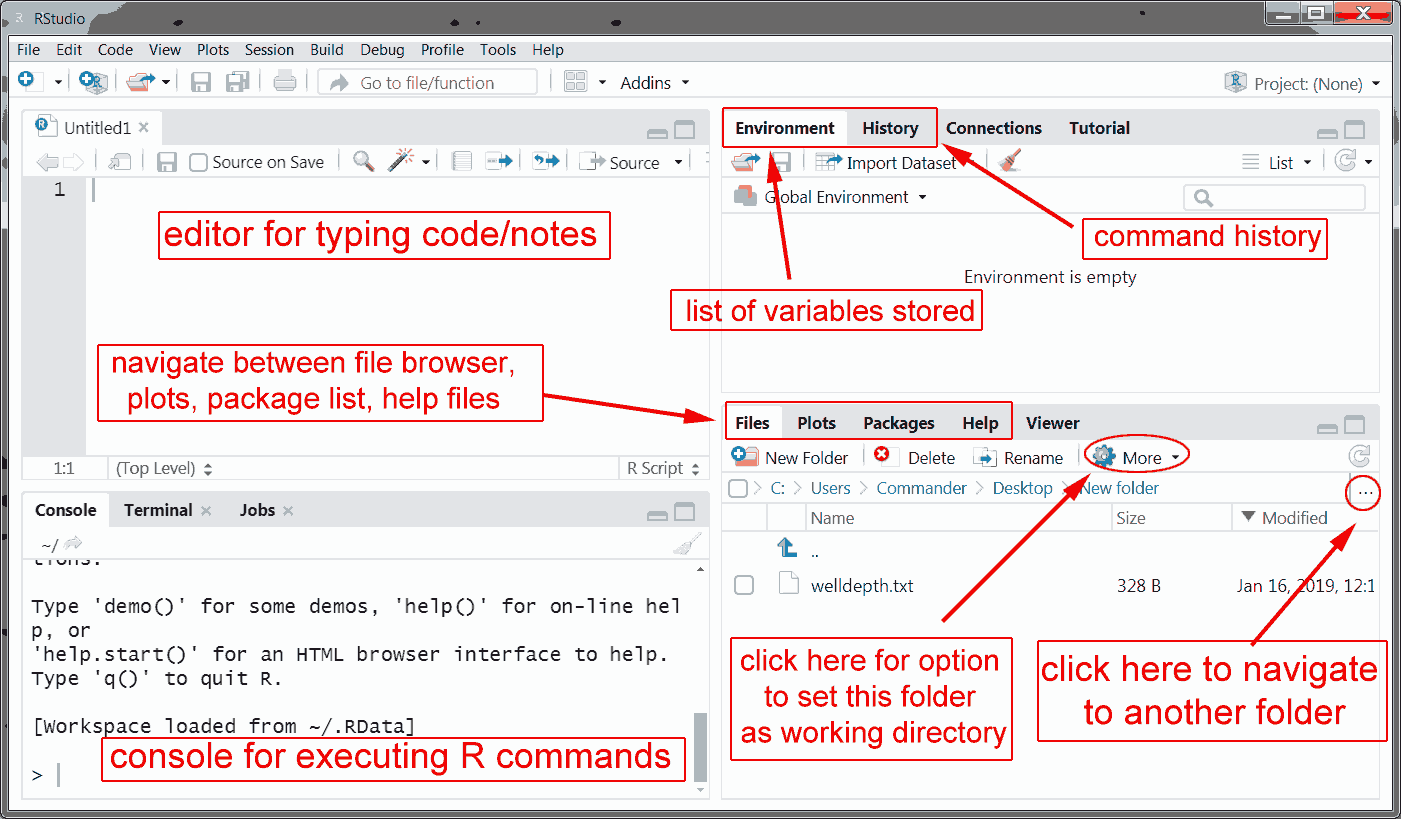
The RStudio user interface.

Using R online through other sources:

Another option for using R statistical software is to use one of the many places online where you can use it through a web browser. There are many such websites.

Here is one website where you can conveniently evaluate R code online from a web browser in any device: https://rdrr.io/snippets/

Another option for having quick access to R (and this is useful for a smartphone) is SageCell at: https://sagecell.sagemath.org/. This website can be used to evaluate commands from a variety of programming languages (including MATLAB and Python). Just select R from the language tab at the lower right of the textbox. If you are familiar with MATLAB, choose the option “Octave”. Octave is basically an open source version of MATLAB and you can run MATLAB code using the Octave language option on SageCell.

1.2 R basics

We can assign variables in R with arrows or equal signs, e.g. x <- 3, 3 -> x, and x = 3 all achieve the same result, setting the variable \(x\) to store the numerical value \(3\). We can perform most arithmetic operations in the usual way, e.g. x+2, 5-x, x/4, x^2, and 5*x. There are also many special functions such as log() (natural log, \(\texttt{log(2)}=\ln(2)\)), sin(), exp() (natural exponentiation, \(\texttt{exp(5)}=e^5\)), etc.

1.2.1 Data structures, vectors, matrices

The basic types of data structures in R include (but are not limited to) numbers, vectors, matrices, and characters.

Here are some additional data structures you might see:
NULL means “empty” but space is reserved for storing something
NA means “nat available” but space is reserved as well
"3" means the string character “3”, not a number. We can coerce this to become a number by as.numeric("3")

Here are some relevant commands:

numeric() creates an empty vector with no dimensions
numeric(length=n) creates a vector of \(n\) zeros
matrix() creates an empty \(1\times1\) matrix with \(\texttt{NA}\) as the entry
matrix(nrows=n,ncol=m) creates an empty matrix of NA’s wtih \(n\) rows and \(m\) columns
c(1,2,3) creates an numeric vector \((1,2,3)\)
0:5 creates an numeric vector \((0,1,2,3,4,5)\)
seq(0,5,by=1) creates an numeric vector \((0,1,2,3,4,5)\)
seq(0,1,by=0.5) creates an numeric vector \((0,0.5,1)\)
seq(0,1,by=0.3) creates an numeric vector \((0,0.3,0.6,0.9)\)
seq(0,1,length.out=4) creates an numeric vector \((0,\frac12,\frac23,1)\)

You access the components of a vector or matrix with square brackets: x[4] is the \(4^{th}\) component of vector \(x\). If \(x\) was a matrix, it would treat it like a vector concatenating the columns together and access the \(4^{th}\) component. We can access the components of a matrix with M[i,j] to get \(M_{ij}\) the component in the \(i^{th}\) row and \(j^{th}\) column.

We can create a \(2\times3\) matrix and store it with the name \(\texttt{M}\) with M <- matrix(nrow=2,ncol=3). Alternatively we can use M <- matrix(ncol=3,nrow=2). Normally for R commands, there is a default order for the arguments you pass through to it, and you don’t need to specify the name of the arguments if you follow that default ordering. If you specify all arguments by name (e.g. nrow=2 and ncol=3), then you can input the arguments in any order. It’s best practice to stick with the default order to develop good habits though.

We can specify a specific matrix in the following way.

M <- matrix(c(1,0,2,3,1,5),nrow=2,ncol=3,byrow=TRUE)

This takes the numeric vector \((1,0,2,3,1,5)\) and constructs the matrix \[\left(\begin{matrix} 1 & 0 & 2\\ 3 & 1 & 5 \end{matrix}\right).\] Alternatively, we can leave off the byrow=TRUE and it will default to constructing the matrix column-by-column. RStudio tends to play nicely with automatically indenting things, so one can put a line break in order to see the rows better in the code.

M <- matrix(c(1,0,2,
              3,1,5),nrow=2,ncol=3,byrow=TRUE)

You can also store characters and strings in vectors and matrices, but once you put in a string, R turns all numerical entries into character data structure as well.

As long as two vectors or two matrices have the same dimensions, you can add or subtract them in the natural way: x+y or A-B. Component-wise multiplication is x*y which will keep the same dimensions but just with components multiplied, and similarly one can do x/y for component-wise division. Matrix multiplication is done with %*% such as x %*% M, but you need to make sure the dimensions are appropriate.

Here are a few other useful commands.
t(M) transpose of matrix or vector \(M\).
inv(M) inverse of matrix \(M\).
dim(x) gives dimensions of object \(x\) (length of vector or number of rows and columns for a matrix).
class(x) gives the class for object \(x\), e.g. it will tell us if it is numeric, character, or a matrix, or some other type of object such as Boolean/logical, etc.

1.3 Installing and using packages in R

It is common for software developers to develop libraries or packages which contain functions and methods. The purpose is the same as a mathematical function. Rather than you rewriting the equation each time, you can program the function and simply call that computer function with a single letter rather than a complicated formula. As an example, R has some base functionality for matrix computations, but in order to raise matrices to exponents, you need to expm package.

Generally to install a package named “packagename” we execute the command install.packages("packagename"). Once a package is installed, in order to use the methods and functions it includes, they must be loaded into R’s active workspace and can be done by executing the command library(packagename).

In order to run the stock simulation code we need to install the packages quantmod and RQuantLib. To do this, execute the commands: install.packages("quantmod") and install.packages("RQuantLib"). You’ll see some output indicating what R is doing, downloading some files, unpacking them, and installing them. Sometimes it may even be compiling some code in the background. Usually it takes a few seconds to minutes to install a new package.

Once a package is installed, in order to use the methods and functions it includes, execute the command library(packagename), e.g. library(quantmod). Notice that installing a package require quotation marks around the package name, but calling it into R’s workspace does not.

1.4 Random variables

R has built in methods for many different random variables. Generally for each random variable there are four methods: dname() (pmf or pdf), pname() (cdf), qname() (quantiles), and rname() (random simulation) where you replace “name” by the name of a particular distribution.

Here are the R names for some common distributions:

Distribution	R name prefix
Binomial	binom
Exponential	exp
Normal	norm
Poisson	pois

1.5 Basics of programming, R scripts

under construction

1.6 Importing datasets into R

Sometimes you might want to import a matrix of vector or otherwise a datset from a website, pdf, or other file format. There are several ways I will discuss getting data into R: text file, csv file (comma separated value), Excel (xls or xlsx), or through the computer’s local clipboard functionality. This is only a small number of input file types that R is capable of handling though.

Import data from text file. To import a single list of data into R, here is the table read method of importing data: 1. Open an Excel spreadsheet.

2. Put a name for your variable/data in the first cell (recommended text only, no spaces or special characters).

3. Type all data values in the column under the name.

4. Save as filetype \(\texttt{Text (MS-Dos) (*.txt)}\)“. Alternatively, open it in MS Notepad, and copy and paste the entire data column, including the name, into Notepad and save it as a *.txt file. Let’s say we saved it as \(\texttt{filename.txt}\).

5. Open R and execute the command: x <- read.table("fileneame.txt", header=T).

Alternatively, if the dataset is small enough that manually typing out the entire list is not a major fuss, we can just use the R command x <- c(x1,x2,x3,...,xn) where \(\texttt{x1,x2,x3,...,xn}\) is our list of actual numerical data values.

I have saved our list of water well depth data is \(\texttt{welldepth.txt}\).

So we can execute: wd <- read.table("welldepth.txt",header=TRUE). This will give our data a data frame" type of tabular structure. A data frame is a specific type of data object in \R. A data frame is composed of multi-variate data, which each individual variable stored as a column. Thenames’’ of each column (which indicate the data stored in that column) are stored at the top of the data frame, in the “header.” To extract just the numerical well depth data, we’ll need to execute x <- wd$well_depth.

The name well\_depth" is the header name for our column of data. In R, the dollar symbol$’’ is used to reference the data stored within a specific column of a data frame. A data frame can have multiple columns with each column given a unique name in the header, e.g. a data frame named \(\texttt{y}\) with columns named \(\texttt{V1, V2, V3}\). We can extract the data from the 2nd column by \(\texttt{y\$V2}\).

Headers: Generally R expects the first horizontal row of your data file to contain the names of the data stored in each column. If your data file has more than two rows of text before the actual data begins, it may cause problems. When loading data you need to pay attention to whether you have copied a header or not.
wd <- read.table("filename.txt", header=TRUE) (reads top line as header)
wd = read.table("filename.txt", header=FALSE) (reads top line as data)

Import data via the file browser. Now that you have gone through the work of manually setting your working directory and importing dataset in with a command line, you will be shown the easy way. Simply click on the three dots in the file pane in RStudio and navigate to the local directory on your computer where the file is stored. Click on the file from within RStuido’s file pane. Then RStudio will automatically give you a preview of the file and dataset and will format the commands necessary to import it, including loading any packages that are necessary. This will work for Excel files, csv files, text files, and many other types of files.

Import data by manually typing. We can also import our well depth data directly by typing it all out separated by commas inside of a c() with:\

x <- c(115,107,114,465,250,220,690,280,
       520,100,450,200,80,500,120,375,
       575,700,80,640,640,680,260,100,
       300,160,440,165,660,120,560,180,
       110,65,120,86,360,100,300,165,
       500,600,600,260,300,620,480,440,
       240,120,420,175,585,240,460,200,
       200,430,482,290,290,620,660,440)

Note that in order to break lines without executing code, use a \(\texttt{Shift-Enter}\) (hold the shift key while pressing the Enter/Return key).

Import data from csv file. If your data is stored as a csv file, it is very much like reading from a text file. Again pay attention to whether or not the top row is a header with names for each of the data variables. d <- read.csv("filename.csv",header=TRUE).

Import data from Excel file. If you have data store in a \(\texttt{xls}\) or \(\texttt{xlsx}\) file, you can import it with the following commands. First we must load the R library “readxl”. An R library is a specific software extension that gives us additional capabilities. You may need to install this package first using the command: install.packages("readxl"). Then once you have confirmed that readxl package is installed, issue the command library(readxl) in order to load the capability into your R session. Then you can finally load the data form the Excel file as follows: d <- read_excel("filename.xlsx",header=TRUE).

Again, pay attention to whether or not your data file include a header row and set the command to either \(\texttt{TRUE}\) or \(\texttt{FALSE}\) appropriately.

Import data from clipboard. A very convenient way to import data is to highlight it on screen and copy it to your computer’s clipboard memory. This works easiest if the data is already formatted nicely in a spreadsheet, but you can copy the data from a pdf, webpage, text file, and many other digital files this way too. It can become tricky as will be illustrated in the example below. Make sure to know whether you are only selecting the data or including a header or name.

Disclaimer: The following works when viewing this pdf in Adobe Reader. If the pdf is opened in other viewing software, this may not work.

If we highlight the list of data above in this pdf and copy it to the computer’s clipboard (right-click and copy or \(\texttt{Ctrl-C}\)), we can import it with the command:read.table("clipboard").

This data will be imported as a “data frame” which is a specific data structure in R and it will be exactly in the format with rows and columns as in this pdf. If the data copied from the clipboard is simply a list of numbers for a single variable, then we will need to extract the numerical data from the data frame and turn it into a numerical list with the following command. This can be tricky to accomplish though.

The following command will turn the data frame (imported via clipboard from copying the well depth data in this pdf within Adobe Reader): x <- as.vector(t(wd)).

Now we have our list of well depths stored as \(\texttt{x}\), and we are ready to analyze it with statistical techniques.

Summary

Summary of notation, formulas, and terminology

under construction