Chapter 13 Brownian motion

Brownian motion is the continuous-time version of the random walk. It is also called the Wiener process. It is one of the most important stochastic process models because it appears as a scaling limit of random walks and because it is a basic model for diffusion and random motion.

A standard Brownian motion is a stochastic process \[ (W_t)_{t\geq0} \] with the following properties:

\(W_0=0\),
for \(s,t\geq0\), \[ W_{t+s}-W_t\sim \mathsf N(0,s), \]
increments over disjoint time intervals are independent.

The third property means that if \[ 0\leq t_1<t_2<t_3<t_4, \] then \[ W_{t_2}-W_{t_1} \] and \[ W_{t_4}-W_{t_3} \] are independent. The same is true for any finite collection of non-overlapping increments.

Brownian motion has continuous sample paths, but they are extremely jagged. They are not smooth in the usual calculus sense.

Standard Brownian motion. A stochastic process \((W_t)_{t\geq0}\) is a standard Brownian motion if \(W_0=0\), it has independent increments, and \[ W_t-W_s\sim\mathsf N(0,t-s) \] for \(0\leq s<t\).

13.1 Distribution at a fixed time

Taking \(s=0\) in the increment distribution gives \[ W_t-W_0\sim\mathsf N(0,t). \] Since \(W_0=0\), \[ W_t\sim\mathsf N(0,t). \] Thus \[ \mathbb E(W_t)=0, \qquad \mathsf{Var}(W_t)=t. \]

The variance increases linearly with time. This matches the intuition that a diffusing particle spreads out more and more as time passes.

13.2 Simulating Brownian motion

To simulate Brownian motion at a finite set of times, choose \[ 0=t_0<t_1<t_2<\cdots<t_k=T. \] Let \[ \Delta t_j=t_j-t_{j-1}. \] The Brownian increments are independent and satisfy \[ W_{t_j}-W_{t_{j-1}}\sim\mathsf N(0,\Delta t_j). \] Thus, to simulate a path, we generate independent normal increments \[ \Delta W_j\sim\mathsf N(0,\Delta t_j) \] and set \[ W_{t_j}=W_{t_{j-1}}+\Delta W_j. \]

Tmax <- 5
dt <- 0.01
t <- seq(0, Tmax, by=dt)

dW <- rnorm(length(t)-1, mean=0, sd=sqrt(dt))
W <- c(0, cumsum(dW))

plot(t, W, type="l", xlab="time", ylab="Brownian motion")
abline(h=0, lty="dashed")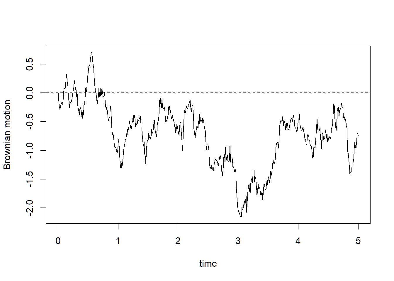

A smaller time step gives a more detailed approximation to the sample path.

13.3 Brownian motion as a diffusion model

Brownian motion can model random movement of a particle in one dimension. It can also be generalized to two or three dimensions by using independent Brownian motions for each coordinate.

The diffusion interpretation is that if a large number of particles are released at the origin, then over time the particles spread out through space. At time \(t\), the location of a single one-dimensional Brownian particle is normally distributed with mean \(0\) and variance \(t\). Its density is \[ \frac1{\sqrt{2\pi t}}e^{-x^2/(2t)}. \] Immediately after release, the particles are highly concentrated near the origin. As time passes, the density spreads out and becomes flatter.

For example, after a cough, there may be a high concentration of aerosol droplets near the mouth. As time passes, the droplets spread out through the air by random motion and other physical forces. Brownian motion is a simplified mathematical model for this kind of spreading.

13.4 Derivation from the simple symmetric random walk

Recall the simple symmetric random walk \[ X_n=\sum_{k=1}^n V_k, \] where \[ \mathbb P(V_k=1)=\mathbb P(V_k=-1)=\frac12. \] Then \[ \mathbb E(V_k)=0, \qquad \mathsf{Var}(V_k)=1. \] Therefore, \[ \mathbb E(X_n)=0, \qquad \mathsf{Var}(X_n)=n. \] By the central limit theorem, for large \(n\), \[ X_n\overset{approx}{\sim}\mathsf N(0,n). \] Equivalently, \[ \frac{X_n}{\sqrt n}\overset{approx}{\sim}\mathsf N(0,1). \]

Now we scale both time and space. Let \(\Delta t>0\) be the size of one time step and let \(\Delta x>0\) be the size of one spatial step. Define a scaled random walk by \[ X_{n\Delta t}=\sum_{k=1}^n V_k\Delta x. \] Then \[ \mathbb E(X_{n\Delta t})=0, \qquad \mathsf{Var}(X_{n\Delta t})=n(\Delta x)^2. \]

To define the process for all times \(t\geq0\), make it a step function. If \[ n\Delta t\leq t<(n+1)\Delta t, \] then set \[ X_t=X_{n\Delta t}. \] Equivalently, \[ X_t=X_{\lfloor t/\Delta t\rfloor\Delta t} =\sum_{k=1}^{\lfloor t/\Delta t\rfloor}V_k\Delta x. \] Thus \[ \mathbb E(X_t)=0, \] and \[ \mathsf{Var}(X_t)=\left\lfloor\frac{t}{\Delta t}\right\rfloor(\Delta x)^2. \]

We want the variance at time \(t\) to converge to \(t\), because Brownian motion satisfies \(\mathsf{Var}(W_t)=t\). To force this, choose \[ \Delta x=\sqrt{\Delta t}. \] Then \[ \mathsf{Var}(X_t)=\left\lfloor\frac{t}{\Delta t}\right\rfloor\Delta t\to t \] as \(\Delta t\to0\).

By the central limit theorem, for fixed \(t\) and small \(\Delta t\), \[ X_t\overset{approx}{\sim}\mathsf N\left(0,\left\lfloor\frac{t}{\Delta t}\right\rfloor\Delta t\right), \] which converges to \[ \mathsf N(0,t). \] Similarly, for \(h>0\), \[ X_{t+h}-X_t\overset{approx}{\sim}\mathsf N(0,h). \] The increments are independent because they are built from disjoint sets of independent random walk steps.

Thus the limiting process has independent normal increments and variance proportional to the length of the time interval. This limiting process is standard Brownian motion.

Scaling from SSRW to Brownian motion. Start with the simple symmetric random walk and scale time by \(\Delta t\) and space by \[ \Delta x=\sqrt{\Delta t}. \] Then, as \(\Delta t\to0\), the scaled random walk converges in distribution to standard Brownian motion.

For any fixed \(t\) and real number \(x\), \[ \mathbb P(X_t\leq x)\to \mathbb P(W_t\leq x) \] as \(\Delta t\to0\), where \[ W_t\sim\mathsf N(0,t). \] That is, \[ \mathbb P(W_t\leq x)=\int_{-\infty}^x \frac1{\sqrt{2\pi t}}e^{-z^2/(2t)}\,dz. \] This kind of convergence is called convergence in distribution.

13.5 Simulating the scaled random walk

The following code simulates the scaled random walk approximation to Brownian motion.

Tmax <- 5
dt <- 0.001
dx <- sqrt(dt)

t <- seq(0, Tmax, by=dt)
steps <- sample(c(-1,1), size=length(t)-1, replace=TRUE)
X <- c(0, cumsum(steps*dx))

plot(t, X, type="l", xlab="time", ylab="scaled random walk")
abline(h=0, lty="dashed")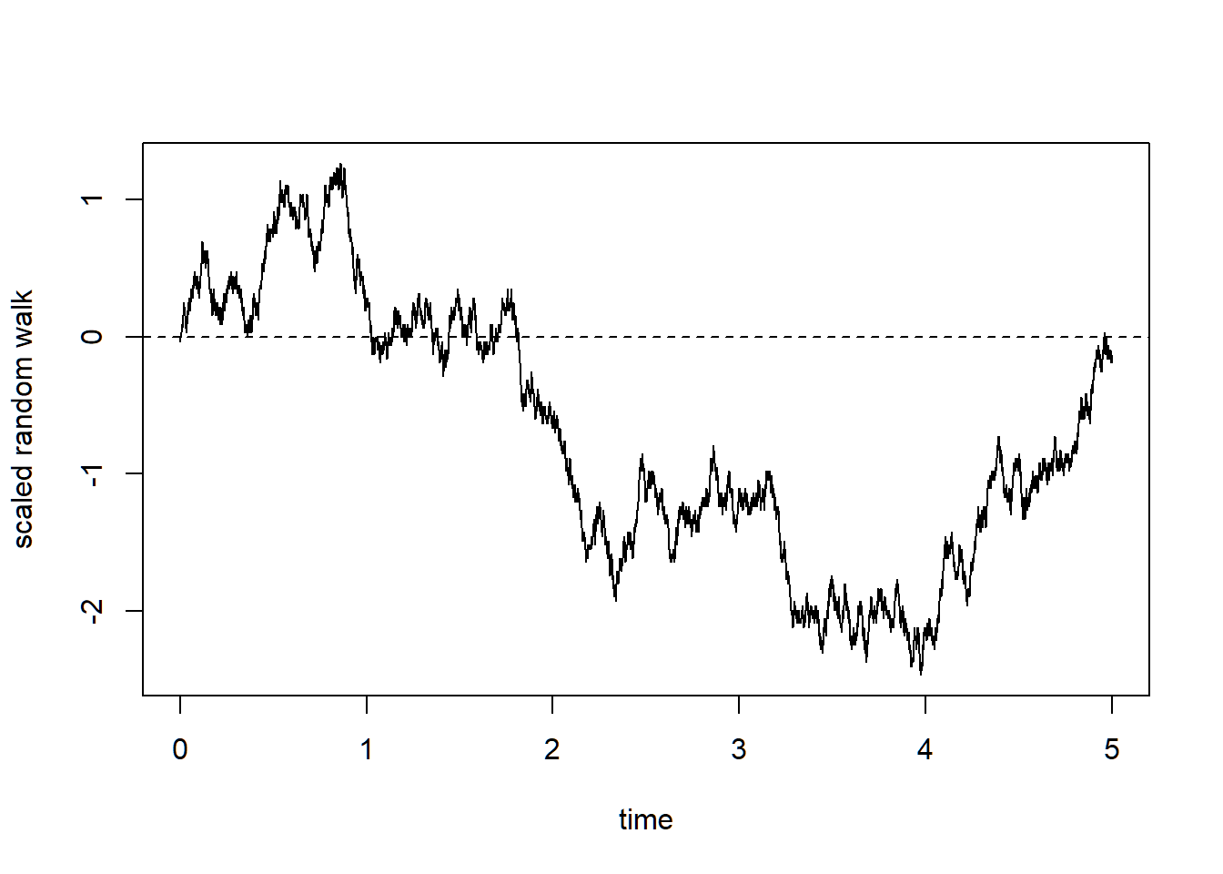

If we make \(\Delta t\) smaller, the paths look more and more like Brownian motion.

13.6 Brownian motion with drift and variance parameter

Standard Brownian motion has mean zero and variance \(t\). A more general Brownian motion with drift \(\mu\) and volatility \(\sigma\) is \[ X_t=\mu t+\sigma W_t. \] Then \[ X_t\sim\mathsf N(\mu t,\sigma^2 t). \] The parameter \(\mu\) controls the average direction of motion, and \(\sigma\) controls the amount of random variation.

Tmax <- 5
dt <- 0.01
t <- seq(0, Tmax, by=dt)
mu <- 0.3
sigma <- 1.2

dW <- rnorm(length(t)-1, mean=0, sd=sqrt(dt))
W <- c(0, cumsum(dW))
X <- mu*t + sigma*W

plot(t, X, type="l", xlab="time", ylab="Brownian motion with drift")
abline(h=0, lty="dashed")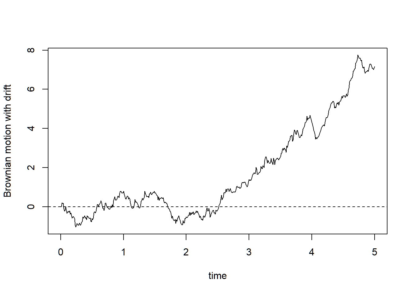

13.7 Geometric Brownian motion and stock prices

A common model for a stock price is geometric Brownian motion. In this model, \[ S_t=S_0\exp\left((\mu-\tfrac12\sigma^2)t+\sigma W_t\right), \] where \(S_0>0\) is the initial stock price, \(\mu\) is the drift parameter, and \(\sigma>0\) is the volatility parameter.

The exponential form ensures that \[ S_t>0 \] for all \(t\geq0\). This is desirable for stock prices because prices should not become negative.

Taking logarithms gives \[ \log(S_t)=\log(S_0)+(\mu-\tfrac12\sigma^2)t+\sigma W_t. \] Thus the log-price is Brownian motion with drift. This is why the model is also called a lognormal stock price model.

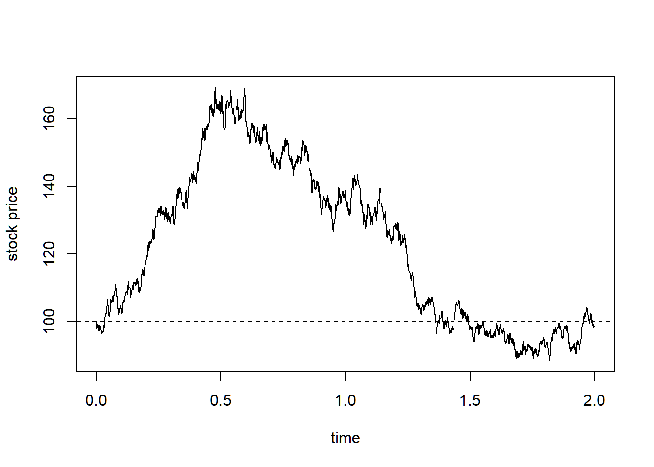
Tmax <- 2
dt <- 0.001
t <- seq(0, Tmax, by=dt)
S0 <- 100
mu <- 0.08
sigma <- 0.25

dW <- rnorm(length(t)-1, mean=0, sd=sqrt(dt))
W <- c(0, cumsum(dW))
S <- S0*exp((mu - 0.5*sigma^2)*t + sigma*W)

plot(t, S, type="l", xlab="time", ylab="stock price")
abline(h=S0, lty="dashed")