Chapter 12 Continuous-time Markov processes
A continuous-time Markov process is the continuous-time analogue of a discrete-time Markov chain. We will focus on the case where the state space is discrete, usually \[ S=\{0,1,2,\ldots,k\} \] or a subset of \(\mathbb Z\). The stochastic process is \[ (X_t)_{t\in[0,\infty)}. \] The process is Markovian if, given the current state, the future evolution does not depend on the past history.
The main new feature in continuous time is that we need to describe both where the process jumps and how long it waits before jumping.
12.1 Transition rates
For states \(i\neq j\), let \[ \lambda_{ij}\geq0 \] be the transition rate from state \(i\) to state \(j\). We write \[ i\to j\quad\text{at rate }\lambda_{ij}. \] The total exit rate from state \(i\) is \[ \nu_i=\sum_{j\neq i}\lambda_{ij}. \] When the process is in state \(i\), it remains there for an exponential length of time with rate \(\nu_i\). Thus the holding time in state \(i\) has distribution \[ \mathsf{Exp}(\nu_i). \] When the process leaves state \(i\), it jumps to state \(j\) with probability \[ \frac{\lambda_{ij}}{\nu_i}. \]
Continuous-time Markov process with transition rates. A continuous-time Markov process on a discrete state space is specified by rates \(\lambda_{ij}\) for \(i\neq j\). From state \(i\), the process waits an exponential time with rate \(\nu_i=\sum_{j\neq i}\lambda_{ij}\) and then jumps to \(j\) with probability \(\lambda_{ij}/\nu_i\).
This construction assumes \(\nu_i<\infty\) for each state \(i\). If \(\nu_i=0\), then state \(i\) is absorbing.
12.2 Two-state example
Suppose the process has states \(0\) and \(1\) and transition rates \[ 0\to1\quad\text{at rate }\beta, \] \[ 1\to0\quad\text{at rate }\delta. \] If \(X_0=0\), then the first jump time to state \(1\) has distribution \[ \tau_1\sim\mathsf{Exp}(\beta). \] After reaching state \(1\), the next jump time back to state \(0\) has distribution \[ \tau_0\sim\mathsf{Exp}(\delta). \] The process alternates between states \(0\) and \(1\), but the amount of time spent in each state is random.
The embedded discrete-time chain just alternates between the two states: \[ T=\begin{pmatrix}0&1\\1&0\end{pmatrix}. \] However, the continuous-time process spends different average amounts of time in the two states unless \(\beta=\delta\).
12.3 Embedded Markov chain
The embedded Markov chain records only the sequence of states visited by the process, ignoring the amount of time spent in each state. Its transition probabilities are \[ T_{ij}=\frac{\lambda_{ij}}{\nu_i},\quad i\neq j, \] and \[ T_{ii}=0 \] unless state \(i\) is absorbing.
The concepts of accessibility, communication, recurrence, and transience for the embedded chain are inherited from discrete-time Markov chains.
12.4 Stationary distributions by holding times
For a finite irreducible continuous-time Markov process, a stationary distribution describes the long-run proportion of time the process spends in each state. One way to understand it is to use the embedded Markov chain.
Suppose the embedded chain has stationary distribution \[ \boldsymbol\pi^*=(\pi_0^*,\pi_1^*,\ldots,\pi_k^*). \] Over a long stretch of transitions, the process visits state \(j\) approximately a proportion \(\pi_j^*\) of the visits. Each time it visits state \(j\), it stays there for an average of \[ \frac1{\nu_j} \] time units. Therefore the long-run proportion of time spent in state \(j\) is proportional to \[ \frac{\pi_j^*}{\nu_j}. \] Normalizing gives \[ \pi_j=\frac{\pi_j^*/\nu_j}{\sum_{\ell=0}^k \pi_\ell^*/\nu_\ell}. \]
Stationary distribution from embedded chain. If \(\boldsymbol\pi^*\) is the stationary distribution for the embedded chain and \(\nu_j>0\) for all states, then the stationary distribution for the continuous-time process is \[ \pi_j=\frac{\pi_j^*/\nu_j}{\sum_\ell \pi_\ell^*/\nu_\ell}. \]
For the two-state chain above, the embedded chain has stationary distribution \((1/2,1/2)\). Therefore \[ \pi_0=\frac{(1/2)(1/\beta)}{(1/2)(1/\beta)+(1/2)(1/\delta)}=\frac{\delta}{\beta+\delta}, \] and \[ \pi_1=\frac{\beta}{\beta+\delta}. \]
12.5 Generator matrix
Another standard way to describe a continuous-time Markov process is with its generator matrix \(G\). The off-diagonal entries are the transition rates: \[ G_{ij}=\lambda_{ij},\quad i\neq j. \] The diagonal entries are negative total exit rates: \[ G_{ii}=-\nu_i. \] Thus each row sums to zero.
A stationary distribution \(\boldsymbol\pi\) satisfies \[ \boldsymbol\pi G=\boldsymbol 0 \] with the normalization condition \[ \sum_j\pi_j=1. \]
Generator matrix stationary equations. A stationary distribution for a finite continuous-time Markov process satisfies \[ \boldsymbol\pi G=\boldsymbol0,\qquad \sum_j\pi_j=1. \] For each state \(j\), this can be written as the equilibrium flow equation \[ \sum_{i\neq j}\lambda_{ij}\pi_i=\nu_j\pi_j. \] The total equilibrium rate into state \(j\) equals the total equilibrium rate out of state \(j\).
12.6 Example with three states
Consider a process with states \(0,1,2\) and transitions \[ 0\to1\text{ at rate }\beta_1, \qquad 1\to0\text{ at rate }\delta_1, \] \[ 0\to2\text{ at rate }\beta_2, \qquad 2\to0\text{ at rate }\delta_2. \] The embedded transition matrix is \[ T=\begin{pmatrix} 0 & \dfrac{\beta_1}{\beta_1+\beta_2} & \dfrac{\beta_2}{\beta_1+\beta_2}\\[8px] 1&0&0\\ 1&0&0 \end{pmatrix}. \] The generator matrix is \[ G=\begin{pmatrix} -(\beta_1+\beta_2)&\beta_1&\beta_2\\ \delta_1&-\delta_1&0\\ \delta_2&0&-\delta_2 \end{pmatrix}. \] Solving \(\boldsymbol\pi G=0\) gives \[ \beta_1\pi_0=\delta_1\pi_1, \qquad \beta_2\pi_0=\delta_2\pi_2. \] Thus \[ \pi_1=\frac{\beta_1}{\delta_1}\pi_0, \qquad \pi_2=\frac{\beta_2}{\delta_2}\pi_0. \] Using \(\pi_0+\pi_1+\pi_2=1\), we get \[ \pi_0=\frac{1}{1+\beta_1/\delta_1+\beta_2/\delta_2}, \] \[ \pi_1=\frac{\beta_1/\delta_1}{1+\beta_1/\delta_1+\beta_2/\delta_2}, \qquad \pi_2=\frac{\beta_2/\delta_2}{1+\beta_1/\delta_1+\beta_2/\delta_2}. \]
12.7 Small-time transition probabilities
If \(X\sim\mathsf{Exp}(\lambda)\), then \[ \mathbb P(X\leq h)=1-e^{-\lambda h}. \] Using the Taylor expansion \[ e^{-\lambda h}=1-\lambda h+O(h^2), \] we get \[ \mathbb P(X\leq h)=\lambda h+O(h^2). \] Thus, over a very short time interval of length \(h\), a transition with rate \(\lambda\) occurs with probability approximately \(\lambda h\).
For a continuous-time Markov process in state \(i\), this means \[ \mathbb P(X_{t+h}=j\mid X_t=i)\approx \lambda_{ij}h, \quad i\neq j, \] and \[ \mathbb P(X_{t+h}=i\mid X_t=i)\approx 1-\nu_i h. \] These small-time approximations are often the easiest way to derive differential equations for expected values.
12.8 Differential equation for the Poisson process mean
For the Poisson process with rate \(\lambda\), let \[ M(t)=\mathbb E(X_t). \] Over a small interval \([t,t+h]\), either there is one event or no event, with probability of two or more events being negligible compared to \(h\). Thus \[ \begin{aligned} \mathbb E(X_{t+h}\mid X_t) &\approx (X_t+1)\lambda h+X_t(1-\lambda h)\\ &=X_t+\lambda h. \end{aligned} \] Taking expectations gives \[ M(t+h)\approx M(t)+\lambda h. \] Therefore, \[ \frac{M(t+h)-M(t)}h\approx\lambda, \] and as \(h\to0\), \[ M'(t)=\lambda. \] Since \(M(0)=0\), we get \[ M(t)=\lambda t. \]
12.9 Birth-death process with immigration
Consider a population process on \(S=\{0,1,2,\ldots\}\) with transitions \[ k\to k+1\quad\text{at rate }k\lambda+\theta, \] and \[ k\to k-1\quad\text{at rate }k\mu, \] for \(k\geq1\). The parameter \(\lambda\) is the per-individual birth rate, \(\mu\) is the per-individual death rate, and \(\theta\) is an immigration rate.
Let \[ M(t)=\mathbb E(X_t). \] For small \(h\), \[ \begin{aligned} \mathbb E(X_{t+h}\mid X_t) &\approx (X_t+1)(X_t\lambda+\theta)h+(X_t-1)(X_t\mu)h\\ &\quad +X_t\big(1-(X_t\lambda+\theta)h-X_t\mu h\big)\\ &=X_t+\big(X_t(\lambda-\mu)+\theta\big)h. \end{aligned} \] Taking expectations and passing to the limit gives \[ M'(t)=(\lambda-\mu)M(t)+\theta. \]
If \(\lambda\neq\mu\), then \[ M(t)=\left(M(0)+\frac{\theta}{\lambda-\mu}\right)e^{(\lambda-\mu)t}-\frac{\theta}{\lambda-\mu}. \] If \(\lambda=\mu\), then \[ M'(t)=\theta, \] so \[ M(t)=M(0)+\theta t. \]
When \(\theta=0\), this reduces to pure exponential growth if \(\lambda>\mu\) and exponential decay if \(\lambda<\mu\).
12.10 Radioactive decay
Radioactive decay can be modeled by the process \[ k\to k-1\quad\text{at rate }k\mu. \] Each of the \(k\) particles has an independent exponential lifetime with rate \(\mu\). If \[ M(t)=\mathbb E(X_t), \] then the birth-death formula with \(\lambda=0\) and \(\theta=0\) gives \[ M'(t)=-\mu M(t). \] Therefore, \[ M(t)=M(0)e^{-\mu t}. \] If \(X_0=N\), then \(M(0)=N\), and \[ \mathbb E(X_t)=Ne^{-\mu t}. \]
The half-life \(\tau_{1/2}\) is the time at which the expected number of particles has been cut in half: \[ Ne^{-\mu \tau_{1/2}}=\frac N2. \] Thus \[ e^{-\mu \tau_{1/2}}=\frac12, \] so \[ \tau_{1/2}=\frac{\log 2}{\mu}. \] Equivalently, \[ \mu=\frac{\log 2}{\tau_{1/2}}. \]
12.11 Chemical reaction model
Consider the reversible chemical reaction \[ A\rightleftharpoons B. \] Suppose individual molecules of type \(A\) convert to \(B\) at rate \(\beta\), and individual molecules of type \(B\) convert to \(A\) at rate \(\alpha\): \[ A\to B\quad\text{at rate }\beta, \] \[ B\to A\quad\text{at rate }\alpha. \]
Let \(N_A\) and \(N_B\) be the initial numbers of molecules of types \(A\) and \(B\), and let \[ N=N_A+N_B \] be the total number of molecules. The total number of molecules is conserved. Let \[ X_t=\#\{A\text{ molecules at time }t\}. \] Then the number of \(B\) molecules is \[ Y_t=N-X_t. \] Therefore we only need to model \(X_t\).
The transitions are \[ X_t\to X_t-1\quad\text{at rate }\beta X_t, \] for \(X_t>0\), and \[ X_t\to X_t+1\quad\text{at rate }\alpha(N-X_t), \] for \(X_t<N\).
This is a finite-state continuous-time Markov process on \[ S=\{0,1,2,\ldots,N\}. \]
12.11.1 Mean behavior
Let \[ M(t)=\mathbb E(X_t). \] For small \(h\), \[ X_{t+h}=X_t+1 \] with probability approximately \((N-X_t)\alpha h\), and \[ X_{t+h}=X_t-1 \] with probability approximately \(X_t\beta h\). Otherwise \(X_{t+h}=X_t\) with the remaining probability. Therefore, \[ \begin{aligned} \mathbb E(X_{t+h}\mid X_t) &\approx (X_t+1)(N-X_t)\alpha h+(X_t-1)X_t\beta h\\ &\quad +X_t\big(1-(N-X_t)\alpha h-X_t\beta h\big)\\ &=X_t+(N-X_t)\alpha h-X_t\beta h. \end{aligned} \] Taking expectations gives \[ M(t+h)-M(t)\approx \big(N\alpha-(\alpha+\beta)M(t)\big)h. \] Thus \[ M'(t)=N\alpha-(\alpha+\beta)M(t). \] Solving this differential equation gives \[ M(t)=M(0)e^{-(\alpha+\beta)t}+\frac{N\alpha}{\alpha+\beta}\left(1-e^{-(\alpha+\beta)t}\right). \] As \(t\to\infty\), \[ M(t)\to \frac{N\alpha}{\alpha+\beta}. \] Thus \[ \frac{\alpha}{\alpha+\beta} \] is the equilibrium proportion of chemical \(A\), and \[ \frac{\beta}{\alpha+\beta} \] is the equilibrium proportion of chemical \(B\).
12.11.2 Simulating the chemical reaction process
The following code simulates the reversible reaction using exponential clocks. This is a basic version of the stochastic simulation algorithm often associated with Gillespie’s method.
# A -> B at rate beta per A molecule
# B -> A at rate alpha per B molecule

alpha <- 1.5
beta <- 2.8
N <- 1000
X0 <- 10
Tmax <- 5

x <- X0
t <- 0
T <- c(t)
X <- c(x)

while (t < Tmax){
  rate_down <- beta*x
  rate_up <- alpha*(N-x)
  total_rate <- rate_down + rate_up
  if (total_rate == 0) break

  wait <- rexp(1, rate=total_rate)
  t <- t + wait
  if (t > Tmax) break

  if (runif(1) < rate_down/total_rate){
    x <- x - 1
  } else {
    x <- x + 1
  }

  T <- c(T, t)
  X <- c(X, x)
}

plot(T, X, type="s", xlab="time", ylab="# molecules of A")
curve(X0*exp(-(alpha+beta)*x) + N*alpha/(alpha+beta)*(1-exp(-(alpha+beta)*x)),
      from=0, to=Tmax, add=TRUE, lwd=3)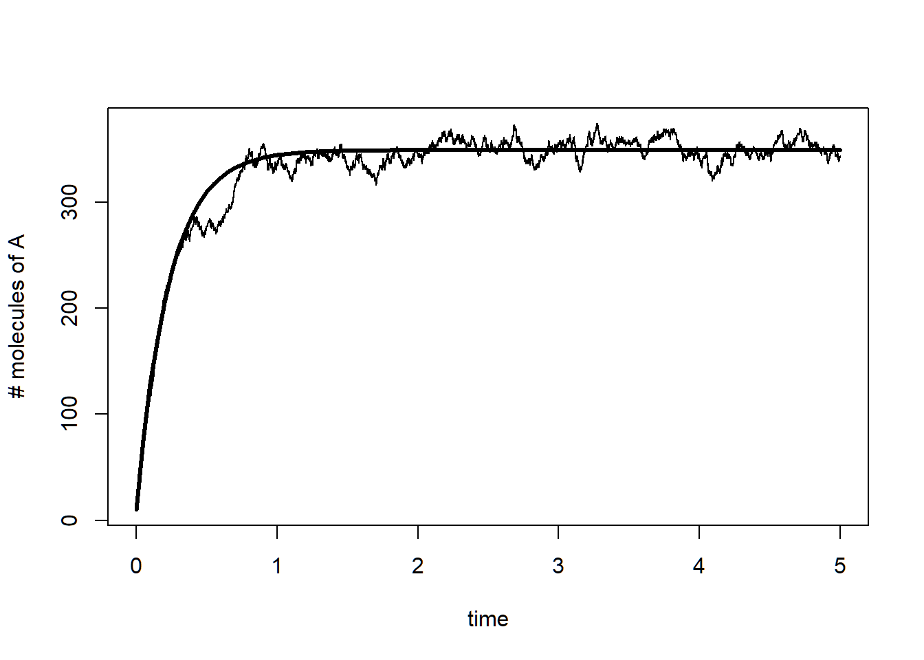
We can repeat the simulation many times and compare the average sample path to the theoretical mean curve.